Rapids to Non-Rapids: The Efficiency Metric Hiding in Every Program You Have Posted

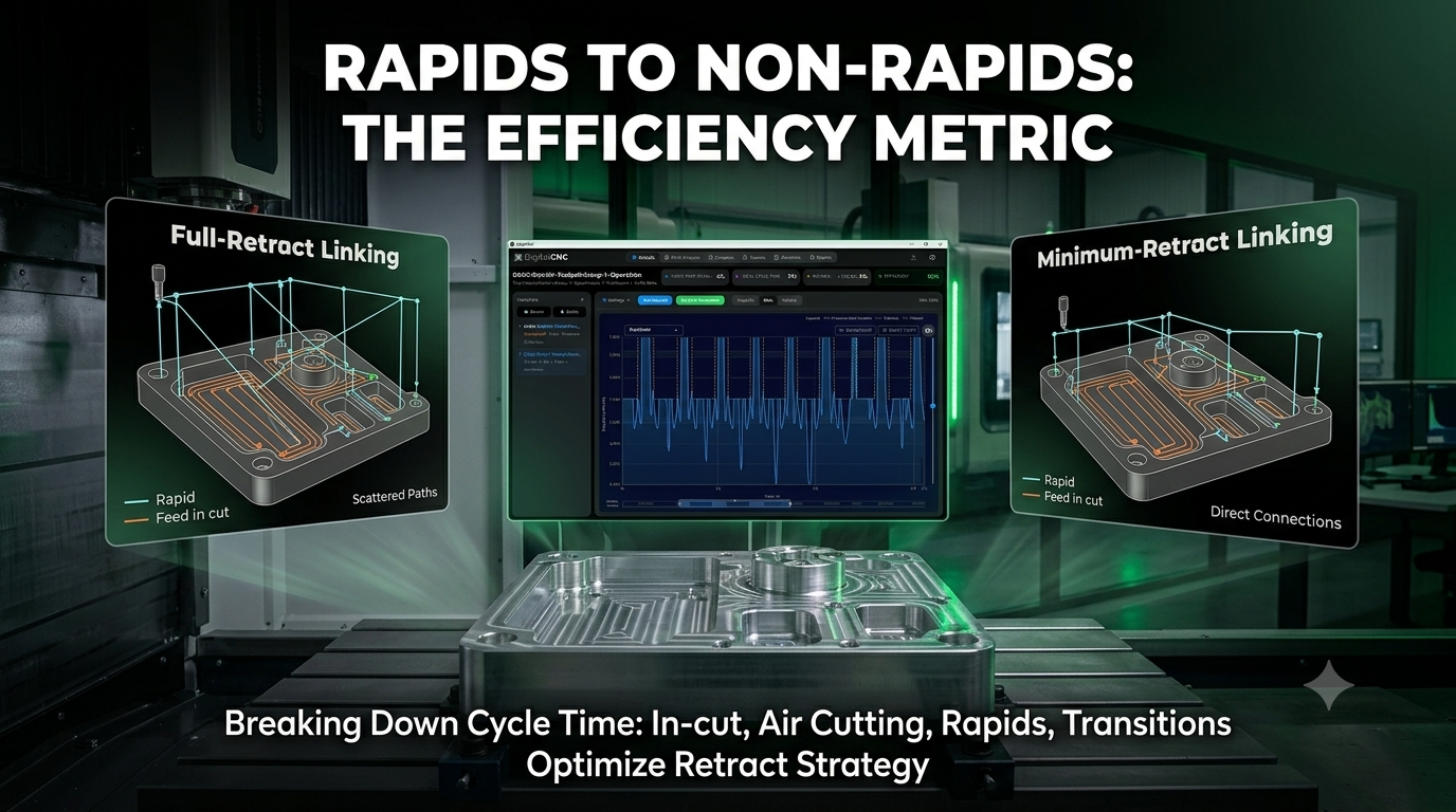
Every CNC program contains two kinds of motion. There is motion that moves the part forward: cutting, finishing, roughing, profiling, drilling and trimming material into shape. Then there is motion that connects the useful work together: retracting, clearing clamps, moving between features, approaching the next cut and positioning safely from one area to another. Both are necessary, but they are not the same.

A machine can look busy while doing very little to the part. It can move quickly, sound productive, and still spend a surprising amount of the cycle travelling through air. That is why the split between rapid motion and feed motion is worth measuring.

The metric is simple: how much of the cycle is spent in rapid traverse compared with how much is spent in feed motion? In G-code terms, this is the difference between rapid moves such as G0 and feed moves such as G1, G2 or G3. In practical terms, it is the difference between repositioning the machine and progressing the part.

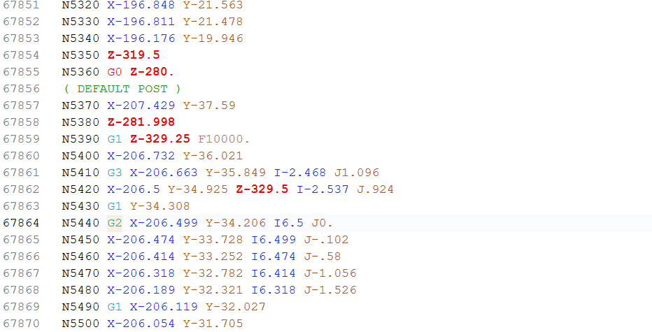
Rapid motion is not waste in the careless sense. Rapids exist because moving between cuts at cutting feed would be worse, and a good program needs safe linking moves, clearance moves and repositioning moves. But rapid motion is still overhead. It is time the machine spends getting ready to cut, moving away from a cut, or travelling to the next cut. It may be necessary, but it does not directly improve the part.

That is the point of the ratio. It gives a programmer, operator or production lead a way to see how much of the cycle is cutting work and how much is connecting tissue. Cycle time tells you what the program costs. The rapid-to-feed split starts to tell you why.

Why This Number Is Easy to Miss

The information is already sitting inside the program. Every motion block declares what kind of move it is, the controller knows whether it is in rapid or feed, and the NC file already contains the raw material needed to separate one from the other. No extra sensor is needed to start asking the question. No spindle load monitoring, no machine connectivity and no new hardware bolted to the side of the control.

At the simplest level, the program can be parsed and the motion blocks separated by mode. How many rapid moves are there? How many feed moves? How much distance is covered in each mode? That first view is useful, but it is not the whole truth.

A distance-based view can be misleading because rapid moves are normally much faster than cutting moves. A long rapid may cover a lot of distance but take very little time, while a short finishing move may cover almost no distance but take much longer. Distance alone can therefore make rapids look worse than they are and make slow feed motion look better than it is. Block count has the same problem. A program may contain many short feed blocks on a freeform surface, or many short rapids between features, so counting blocks tells you something about program structure but not about the real cost.

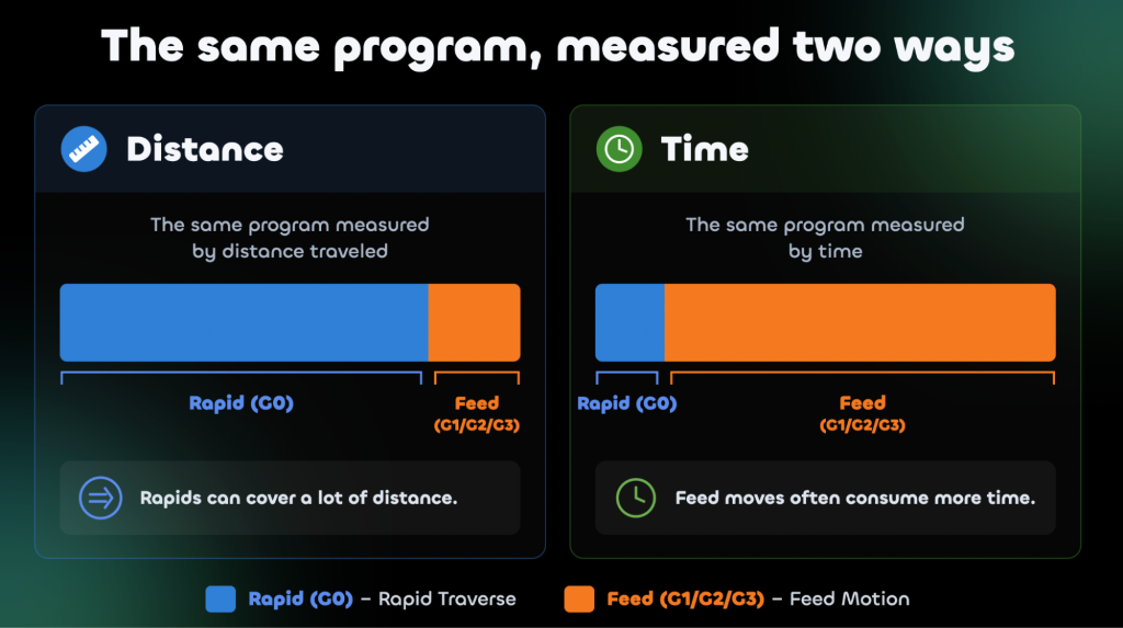
Still, this first view is useful for spotting obvious problems. If a program contains hundreds of retracts to a high safe plane, or constant repositioning between scattered features, the structure will show up quickly. It may not give you the final answer, but it tells you where to look.

Measuring It More Honestly

The next level is time. Instead of counting blocks or measuring distance, each move can be converted into an estimated time, with feed moves timed using the programmed feed rate and rapid moves timed using the machine’s rapid traverse rate. That is closer to reality, and it is how a lot of cycle time estimating already works. But there are two big catches.

The first is rapid motion. A machine does not instantly reach its maximum rapid rate. On short rapid moves, the axis may spend most of the move accelerating and decelerating, and it may never get anywhere near the rapid rate printed in the machine specification. That means lots of short rapids can cost far more time than the numbers suggest. The expensive part is not always the distance; it is the repeated stop-start motion.

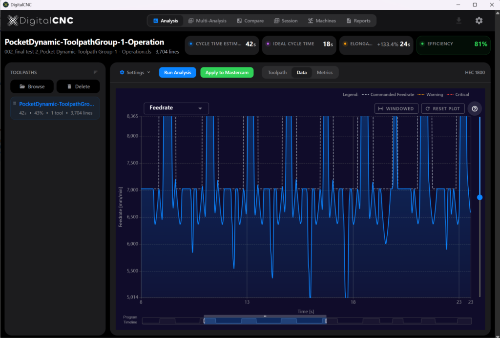
The second catch is feed motion. The machine does not always hold the programmed feed rate. Through dense geometry, tight changes of direction, small segments or five-axis movement, the controller may slow the machine down to stay within acceleration, jerk and axis limits. To the operator, this is familiar: the program says one feed, the control shows another. The machine is not disobeying the code; it is executing the code within the limits of the machine. This is the same behaviour that sits behind look-ahead and controller smoothing. The controller plans velocity across the geometry it can see, and where the geometry demands more than the machine can deliver, the controller resolves the conflict in favour of the machine. The programmed feed rate is a ceiling, not a promise.

So a time estimate based only on programmed feeds and headline rapid rates describes a machine that does not really exist. It assumes every rapid reaches full speed, every feed move holds programmed feed and every transition costs nothing. Real machines do not work like that.

The most honest rapid-to-feed ratio comes from execution-level timing: what the machine actually does with the program. That means real achieved feed rates, real acceleration behaviour, real transition time and real controller decisions. That information can be found in two places. One is after the job has run, by measuring what happened on the machine. The other is before the job runs, by simulating the program against the real kinematics of the specific machine and controller. The first method costs production time before the lesson is learned. The second gives the programmer and operator a better picture before the spindle turns.

The Blind Spot: Feed Motion Is Not Always Cutting

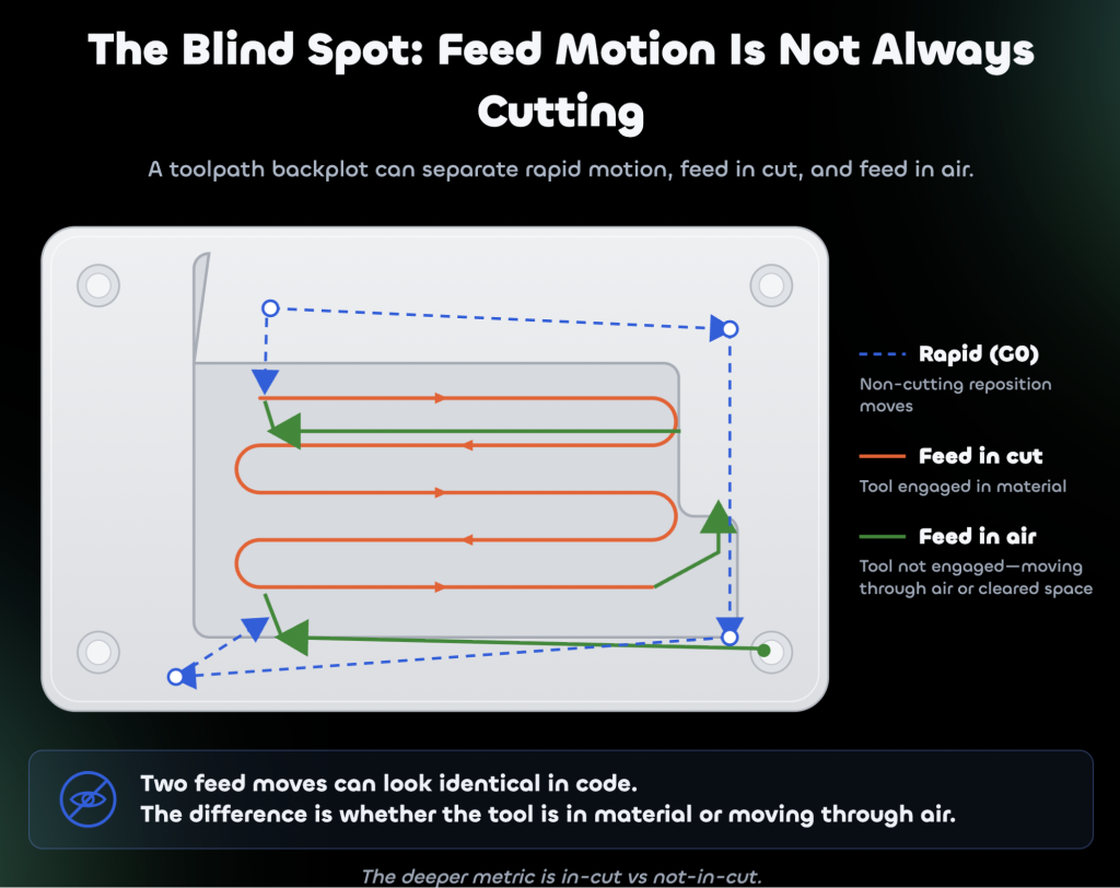
There is one more important point. Rapid versus feed is useful, but it is not the complete picture, because not every feed move is an in-cut move. Programs often contain feed moves where the tool is cutting air. Lead-ins, lead-outs, safety links, positioning moves output at feed, approach moves, and passes through material that has already been removed can all happen in feed mode.

This is where the simple rapid-to-feed split can flatter a program. A cycle may show a high feed-motion percentage, but some of that feed time may still be non-cutting time. The machine is moving slowly, but the tool is not doing useful work. That is the most expensive kind of air cutting: not rapid, not productive, just slow.

So the deeper metric is not only rapid versus feed. It is in-cut versus not-in-cut. Knowing the difference requires more than reading the code, because the code does not say where the material is. A feed move through air and a feed move through stock look identical in the program. Separating them means knowing the state of the stock at every point in the cycle, which is why this deeper split is harder to reach than the first one.

The rapid-to-feed ratio is the accessible first approximation. It is easy to understand and easy to start measuring. But the blind spot should be known from the start: some feed time is productive, and some feed time is just overhead wearing a better disguise.

Where the Time Usually Hides

Once you start looking for non-cutting time, certain areas show up again and again.

The first is retract strategy. Many programs retract to a safe plane after every feature, every pass or every reposition. That is often the conservative default, especially in templates built to avoid crashes across a wide range of setups. The problem is that every retract looks harmless on its own: one move up, one move across, one move down. But across a mature production program, those moves can happen hundreds of times, and together they can become one of the largest recoverable blocks of time in the cycle.

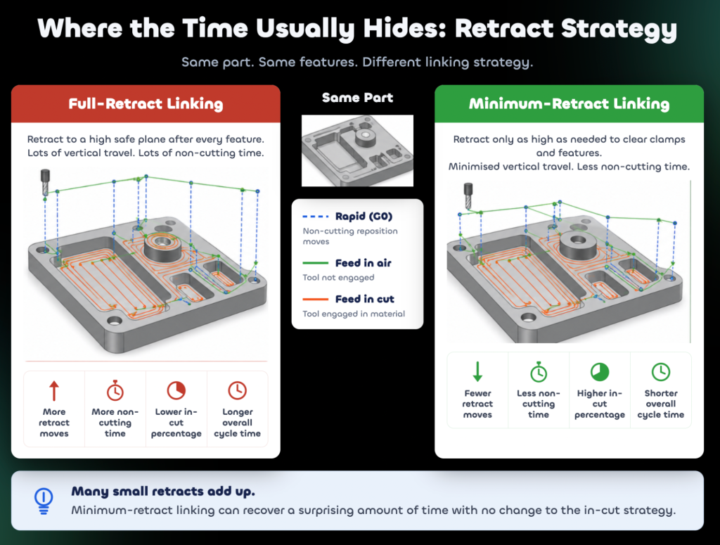
Minimum-retract linking can help where the part, fixture, clamps and tool length make it safe, and the key word is safe. A saved linking move is never worth a damaged cutter or a scrapped billet. But when a lower linking height is safe, the rapid-to-feed ratio gives you a way to measure the effect before and after. It turns “this feels better” into “this removed measurable overhead.”

The second hiding place is short rapid moves. Operators often notice long rapids because they are visible: the machine moves across the envelope and everyone can see it. But the expensive rapids are often the small ones. A program with many short hops may never let the machine reach full rapid speed, and each hop carries an acceleration and deceleration penalty. The machine is constantly starting, stopping, checking position and changing mode. That dead time does not always stand out when watching the program run, but it adds up.

The third area is mode transitions. Moving from rapid to feed, feed to rapid, or one controlled state to another can introduce small delays. Depending on the controller settings, exact-stop behaviour, tolerance mode and machine configuration, the machine may pause, settle or verify position before continuing. Each event is tiny, but a full program may contain thousands of them. This is why the instinct should not simply be to shorten the rapid distance. The better instinct is often to reduce unnecessary transitions.

The fourth area is sequencing. The order in which features are machined affects how much repositioning is needed, and two programs can cut the same features with the same tools and still have very different amounts of linking motion. Tool grouping matters too. Doing all sensible work for a tool before changing it can reduce tool change and repositioning overhead, and ordering features so the machine does not bounce around the part unnecessarily can reduce connecting moves. The ratio makes those choices measurable instead of habitual.

The fifth area is CAM strategy. Two toolpaths can produce the same surface and still carry very different amounts of overhead. One strategy may cut continuously with clean linking, while another constantly retracts, repositions and re-enters. On the screen, both may look acceptable. At the machine, one may carry a much larger non-cutting load. That is why strategy comparisons should not only look at stepover, feed, spindle speed and surface finish. They should also look at how much time the machine spends between useful cuts.

The Ratio Is Comparative, Not Universal

There is no perfect rapid-to-feed target. A roughing operation with many islands, clamps or deep pockets will naturally need more retracts than a continuous finishing pass. A five-axis trimming operation will behave differently from a drilling cycle, and a large aerospace structure will not have the same motion profile as a small prismatic bracket. So the number should not be used as a universal score.

Its strength is comparison. Compare two versions of the same program, two strategies for the same feature, the first posted version with the revised version, or last batch with this batch. When the geometry is broadly the same, changes in the ratio tell you something useful: whether the program has become more efficient, or whether time has simply moved around.

That is where the metric becomes practical. It helps answer questions operators and programmers already ask. Why did this cycle run longer than expected? Did the revised linking strategy actually save anything? Are we losing time in cutting, in air, or between cuts? Is the machine slow because the process is heavy, or because the program keeps sending it on errands? That last one matters more than people like to admit.

Why Operations Should Care Too

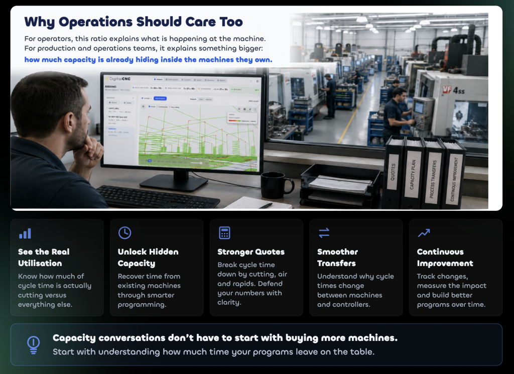
For operators, this ratio explains what is happening at the machine. For production and operations teams, it explains something bigger: how much capacity is already hiding inside the machines they own.

Spindle-on time is a common measure, but it is blunt. A machine can have the spindle running while cutting metal, trimming composite, moving through air, feeding into a lead-in, or repositioning safely above the job, and from a utilisation report those minutes may all look the same. They are not the same. The in-cut share of cycle time is a more honest process-level measure. It shows how much of the cycle is actually advancing the part and how much is overhead required to connect that work together.

That matters because capacity conversations often jump straight to capital expenditure. We need another machine. Maybe. But the first question should be: what are the current programs leaving on the table? If a facility can identify that a meaningful share of cycle time is non-cutting motion, some of that time may be recoverable through programming changes alone. Not all of it, because safe clearance, fixturing, tool changes and machine limits still exist. But some of it. And recovering time from existing programs is very different from buying another machine, hiring another shift, or accepting longer lead times.

The ratio also helps with quoting and process transfer. A decomposed cycle time is easier to defend than a single number, and if a quote is challenged, it helps to know whether the time sits in cutting, linking, tool changes, air moves or machine-limited motion. The same applies when work moves between machines. If a program is transferred and the cycle changes, the split helps explain why. Did the new machine lose time in rapid moves? Did the controller slow down in feed? Did the rotary axes become the bottleneck? Did transitions behave differently? A single cycle time cannot answer those questions. A decomposed cycle can. It gives programmers, operators and operations leads a shared number instead of three different opinions about the same lost minutes.

How Programs Should Be Evaluated

Cycle time is the number everyone tracks. The problem is that cycle time on its own is hard to improve, because it tells you the total cost of the program but not where the cost lives. The rapid-to-feed ratio starts the decomposition. The in-cut versus not-in-cut split completes it. Together, they turn cycle time from a single lump of minutes into something that can be understood and improved.

If a cycle runs over estimate, the question becomes clearer. Was the extra time in cutting? Was it in air cutting? Was it in rapid positioning or short transitions? Was it caused by the controller slowing through dense geometry, or by retract strategy, sequencing and toolpath structure? Those are useful questions because they point to action.

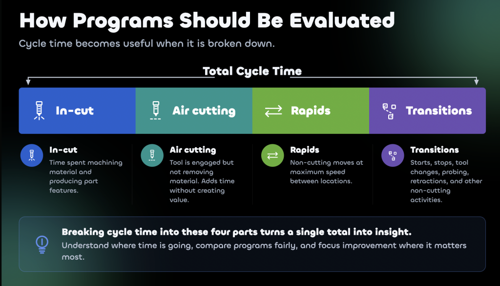
Producing that decomposition honestly requires knowing what the machine actually does with the program, since both rapid and feed timing are set by the machine and controller rather than by the values written in the code. At DigitalCNC, this is part of the problem we work on: modelling how a specific machine and controller will execute an NC program before it runs, so the programmer can see the real motion split before machine hours are spent.

Every programmer has watched a machine glide through a long reposition and felt the program was efficient because it looked busy. But being busy is not the same as being productive. The ratio replaces the feeling with a number. The machine has always known how much of the cycle was cutting. Now the programmer does too.